

Unit 3 AP Macro Notes: Study AD-AS, Output Gaps & Policy

Studying national income and price determination means understanding how spending, production, and the overall price level interact. Well-organized unit 3 ap macro notes help you connect aggregate demand, short-run aggregate supply, long-run aggregate supply, fiscal policy, and economic fluctuations instead of memorizing each graph or formula separately.
This guide reviews the core AP Macroeconomics Unit 3 concepts, explains how to read AD-AS models, covers multiplier calculations and output gaps, and shows how to organize your class materials with Lynote AI Note Generator. Use it alongside your current course framework, teacher materials, and official AP resources.
TL;DR: What to Focus on in AP Macro Unit 3
- Understand what shifts aggregate demand (AD), short-run aggregate supply (SRAS), and long-run aggregate supply (LRAS).
- Distinguish movements along a curve from shifts of a curve.
- Identify short-run equilibrium, potential output, recessionary gaps, and inflationary gaps.
- Practice the spending multiplier and tax multiplier.
- Explain how fiscal policy changes aggregate demand.
- Understand how wages and input prices can shift SRAS during long-run adjustment.
- Practice interpreting graphs and explaining cause-and-effect relationships.
What Is Unit 3 in AP Macroeconomics?
Unit 3 is commonly titled National Income and Price Determination. It focuses on how aggregate spending and aggregate production determine real output and the overall price level in the short run, and how the economy adjusts toward long-run equilibrium.
The unit connects the expenditure model to the aggregate demand and aggregate supply framework. It also examines how changes in spending, production costs, and government policy can create or close output gaps.
Main Topics in Unit 3
Use your current AP course framework and class syllabus to confirm the exact topic sequence. Core areas include aggregate demand, short-run aggregate supply, long-run aggregate supply, macroeconomic equilibrium, output gaps, the multiplier effect, fiscal policy, and long-run adjustment.
A useful set of AP Macro notes should explain each model, identify what causes a curve to shift, and predict the effect on real GDP and the price level.
Aggregate Demand: Understanding the AD Curve
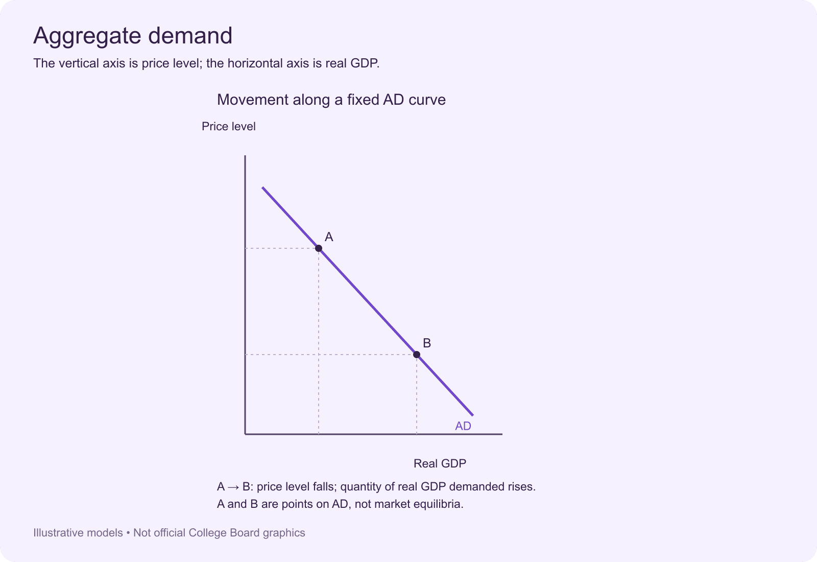
Aggregate demand represents the total quantity of final goods and services demanded in an economy at different overall price levels, holding other relevant factors constant. The AD curve slopes downward, showing an inverse relationship between the price level and the quantity of real output demanded.
The components of aggregate demand are commonly summarized as:
AD = C + I + G + (X − M)
Here, C represents consumption, I represents investment, G represents government purchases, and X minus M represents net exports. Government purchases should be distinguished from transfer payments, which are not directly counted as purchases of current goods and services in GDP.
Why Does the AD Curve Slope Downward?
Three commonly taught effects help explain the downward slope:
- Wealth effect: A lower price level can increase the purchasing power of some money-denominated assets, encouraging consumption.
- Interest-rate effect: A lower price level can reduce transaction demand for money and put downward pressure on interest rates, encouraging borrowing and investment under the model's assumptions.
- Exchange-rate effect: Changes in domestic interest rates can affect the currency's value and influence exports and imports.
These effects explain a movement along the AD curve when the overall price level changes. They are different from the factors that shift the entire AD curve.
What Shifts Aggregate Demand?
Aggregate demand shifts when a determinant other than the current price level changes.
| AD Determinant | Possible Increase in AD | Possible Decrease in AD |
|---|---|---|
| Consumption | Higher consumer confidence or wealth | Lower confidence or wealth |
| Investment | Improved business expectations | Reduced expected profitability |
| Government Purchases | Higher government purchases | Lower government purchases |
| Net Exports | Higher foreign demand, other things equal | Lower foreign demand, other things equal |
When AD shifts right, real GDP and the price level generally rise in the short run, assuming an upward-sloping SRAS curve. When AD shifts left, real GDP and the price level generally fall in the short run.
Short-Run Aggregate Supply: Production Costs and Output
Short-run aggregate supply represents the quantity of real output firms are willing and able to produce at different price levels when some input prices, such as nominal wages, are sticky. The SRAS curve generally slopes upward because firms may find production more profitable when output prices rise before all input costs adjust.
What Shifts SRAS?
SRAS shifts when production costs or other supply conditions change independently of the current price level.
| Factor | Effect on SRAS |
|---|---|
| Lower nominal wages | Shifts SRAS right |
| Higher nominal wages | Shifts SRAS left |
| Lower raw-material or energy costs | Shifts SRAS right |
| Higher raw-material or energy costs | Shifts SRAS left |
| Improved productivity | Shifts SRAS right |
| Supply disruption | Often shifts SRAS left |
A rightward SRAS shift means firms are willing to produce more at each price level. A leftward shift means firms are willing to produce less at each price level.
Movement Along SRAS vs. Shift of SRAS
A change in the overall price level causes a movement along an existing SRAS curve. A change in nominal wages, input prices, productivity, or another production condition shifts the entire curve.
Before moving a curve on an exam graph, identify whether the question describes a change in the price level or a change in a determinant of aggregate supply.
Long-Run Aggregate Supply and Potential Output
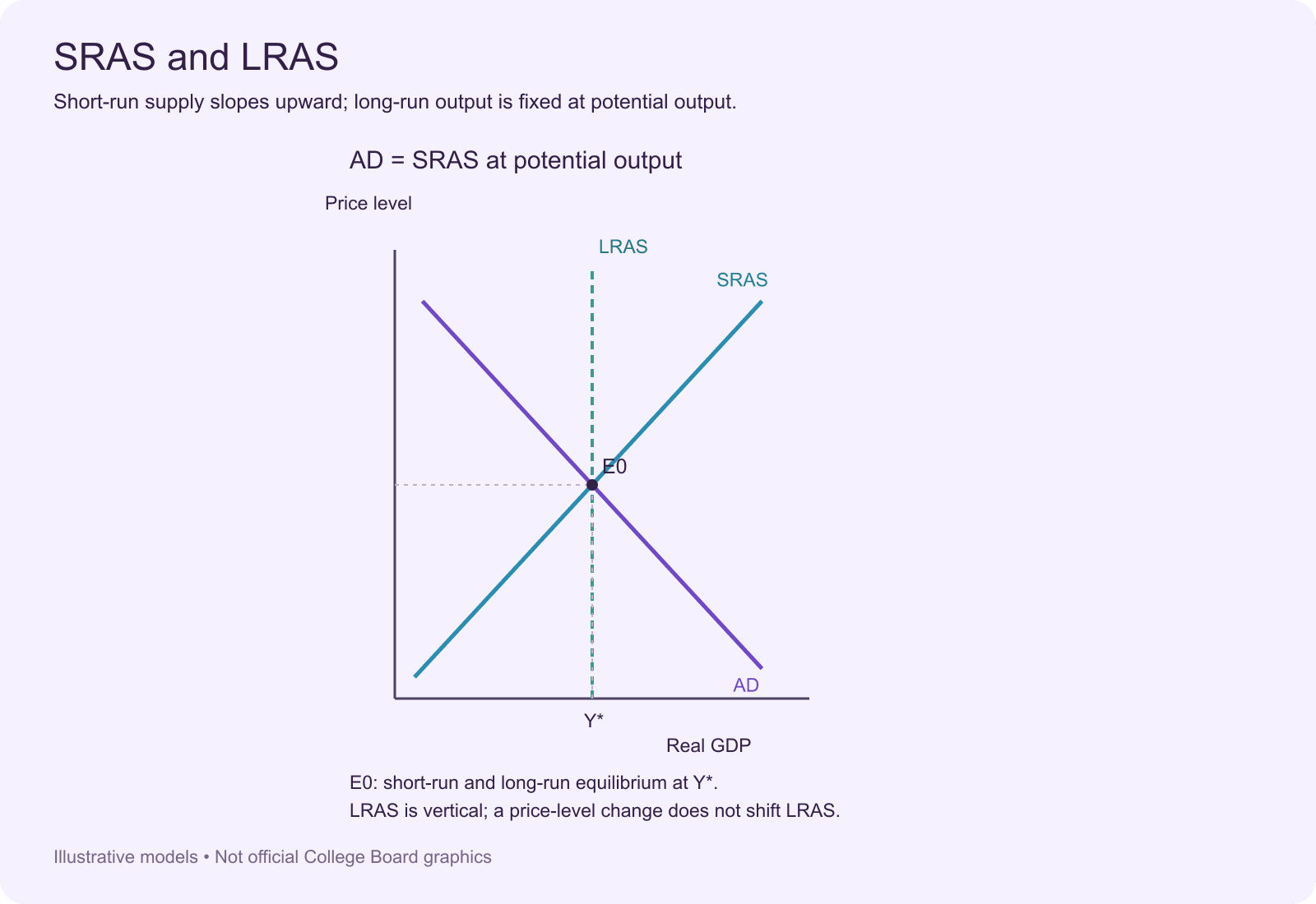
Long-run aggregate supply represents the economy's potential output when labor and other resources are employed at their normal, sustainable levels. In the standard AP model, LRAS is drawn as a vertical line at potential real GDP because the price level does not determine the economy's long-run productive capacity.
Potential output depends on the quantity and quality of resources and the economy's productive technology and institutions. Changes in human capital, physical capital, natural resources, or technology can shift LRAS.
What Shifts LRAS?
- More physical capital: Investment can increase productive capacity over time.
- Improved human capital: Education, training, and experience can raise worker productivity.
- Technological progress: Better production methods can increase potential output.
- Changes in available resources: Labor force growth or access to productive resources can affect capacity.
- Productivity-enhancing institutions: Conditions that improve resource allocation can influence long-run output.
An increase in productive capacity shifts LRAS to the right. A decrease in productive capacity shifts LRAS to the left.
Short-Run and Long-Run Macroeconomic Equilibrium
Short-run macroeconomic equilibrium occurs where AD and SRAS intersect. This intersection determines the short-run equilibrium price level and real GDP.
Long-run equilibrium occurs when AD, SRAS, and LRAS intersect at the same point. At that point, real GDP equals potential output, and cyclical unemployment is absent in the simplified model.
How to Read an AD-AS Graph
- Identify the initial intersection of AD and SRAS.
- Locate LRAS to determine potential output.
- Identify the event described in the question.
- Decide whether AD, SRAS, or LRAS shifts.
- Mark the new short-run equilibrium.
- Compare the new real GDP with potential output.
- Explain the change in the price level and output.
Always label both axes: the vertical axis represents the overall price level, and the horizontal axis represents real GDP. Clearly mark the original and new curves so the direction of each change is easy to follow.
Recessionary and Inflationary Gaps
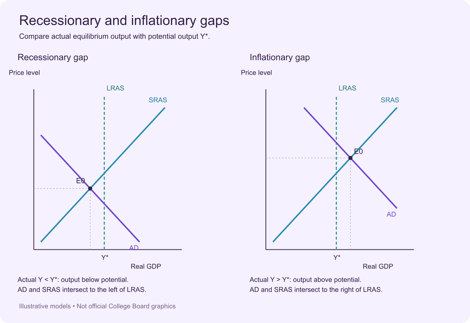
An output gap occurs when short-run equilibrium real GDP differs from potential output. The direction of the gap helps explain unemployment and the pressure for wages and input prices to adjust.
Recessionary Gap
A recessionary gap occurs when short-run equilibrium real GDP is below potential output. In the simplified model, cyclical unemployment is positive and the unemployment rate is above the natural rate.
A leftward shift in AD can create a recessionary gap. Lower aggregate spending reduces equilibrium output in the short run, and the economy produces below its sustainable capacity.
Inflationary Gap
An inflationary gap occurs when short-run equilibrium real GDP is above potential output. The economy is producing beyond its sustainable level, and unemployment is below the natural rate in the simplified model.
A rightward shift in AD can create an inflationary gap. Strong aggregate spending increases short-run output, but resource constraints can create upward pressure on wages and other input costs.
Recessionary Gap vs. Inflationary Gap
| Feature | Recessionary Gap | Inflationary Gap |
|---|---|---|
| Real GDP | Below potential output | Above potential output |
| Unemployment | Above natural rate | Below natural rate |
| Labor Market | Weaker demand for labor | Stronger demand for labor |
| Wage Pressure | Downward pressure over time | Upward pressure over time |
| Typical Long-Run SRAS Adjustment | Rightward | Leftward |
The Spending Multiplier and Tax Multiplier
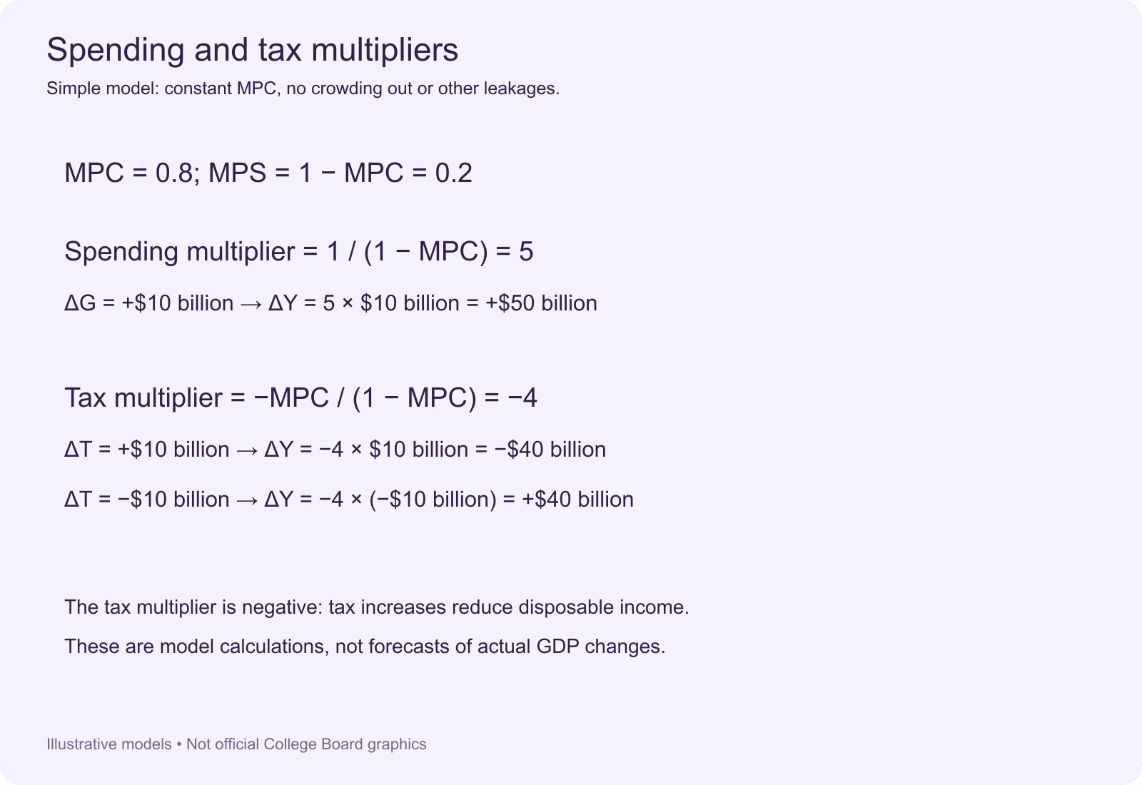
The multiplier effect explains why an initial change in autonomous spending can lead to a larger total change in equilibrium output. One person's spending becomes another person's income, and part of that additional income may be spent again.
The Spending Multiplier
In the simple model, the spending multiplier is:
Spending Multiplier = 1 / (1 − MPC)
MPC is the marginal propensity to consume, or the fraction of an additional dollar of disposable income that households spend. In the simplified model, the marginal propensity to save (MPS) and MPC add up to one.
Example: If MPC is 0.8, the spending multiplier is 5. An initial $10 billion increase in autonomous spending could increase equilibrium output by up to $50 billion in this simplified model, assuming the model's conditions hold.
The Tax Multiplier
A change in taxes affects disposable income and therefore consumption. In the simple model, the tax multiplier is:
Tax Multiplier = −MPC / (1 − MPC)
The tax multiplier is negative because an increase in taxes reduces disposable income and consumption, other things equal. A tax cut has the opposite direction of effect.
Example: If MPC is 0.8, the tax multiplier is -4. A $10 billion tax increase could reduce equilibrium output by $40 billion in the simplified model. A $10 billion tax cut could increase it by $40 billion, assuming the same conditions.
Spending Multiplier vs. Tax Multiplier
| Feature | Spending Multiplier | Tax Multiplier |
|---|---|---|
| Formula | 1 / (1 - MPC) | -MPC / (1 - MPC) |
| Initial Change | Autonomous spending | Taxes |
| Direction | Positive | Negative |
| Equal-Sized Increase | Larger modeled effect on output | Smaller absolute effect on output |
| Main Channel | Direct spending and subsequent consumption | Disposable income and consumption |
These formulas are simplified model results. In real economies, saving, taxes, imports, price changes, interest rates, and policy responses can affect the final impact.
Fiscal Policy and Aggregate Demand
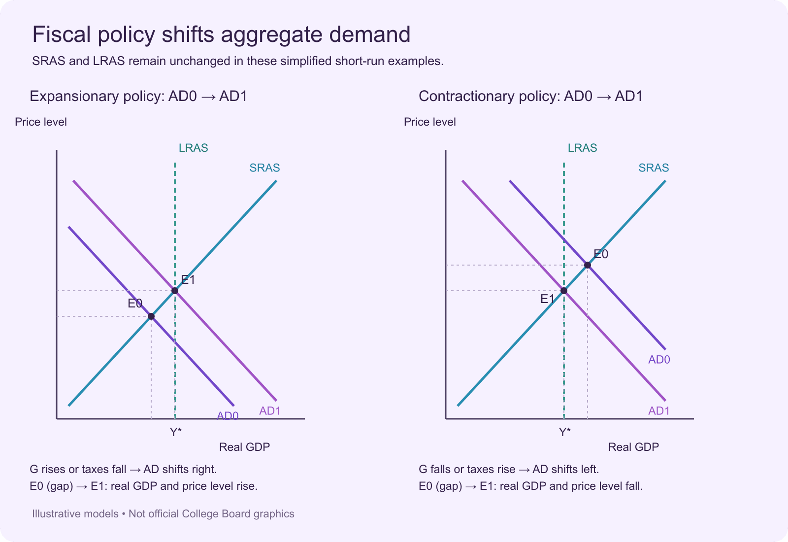
Fiscal policy refers to changes in government purchases and taxes intended to influence economic activity. In the AD-AS framework, fiscal policy can shift aggregate demand and affect short-run real GDP and the price level.
Expansionary Fiscal Policy
Expansionary fiscal policy is generally used to address a recessionary gap. It can involve increasing government purchases, reducing taxes, or a combination of both.
Higher government purchases directly increase aggregate demand. Tax reductions can raise disposable income and consumption, depending on how households respond.
In the AD-AS model, expansionary fiscal policy shifts AD to the right. In the short run, real GDP and the price level generally rise, other things equal.
Contractionary Fiscal Policy
Contractionary fiscal policy can be used to reduce an inflationary gap. It may involve decreasing government purchases, increasing taxes, or combining both measures.
Lower government purchases directly reduce aggregate demand. Higher taxes can reduce disposable income and consumption, depending on household behavior.
In the AD-AS model, contractionary fiscal policy shifts AD to the left. In the short run, real GDP and the price level generally fall, other things equal.
Fiscal Policy Comparison
| Policy | Government Purchases | Taxes | AD Direction | Common Application |
|---|---|---|---|---|
| Expansionary | Increase | Decrease | Right | Recessionary gap |
| Contractionary | Decrease | Increase | Left | Inflationary gap |
Students should also distinguish discretionary policy changes from automatic stabilizers, which change government revenue or transfer spending as economic conditions change without a new legislative action.
Long-Run Adjustment in the AD-AS Model
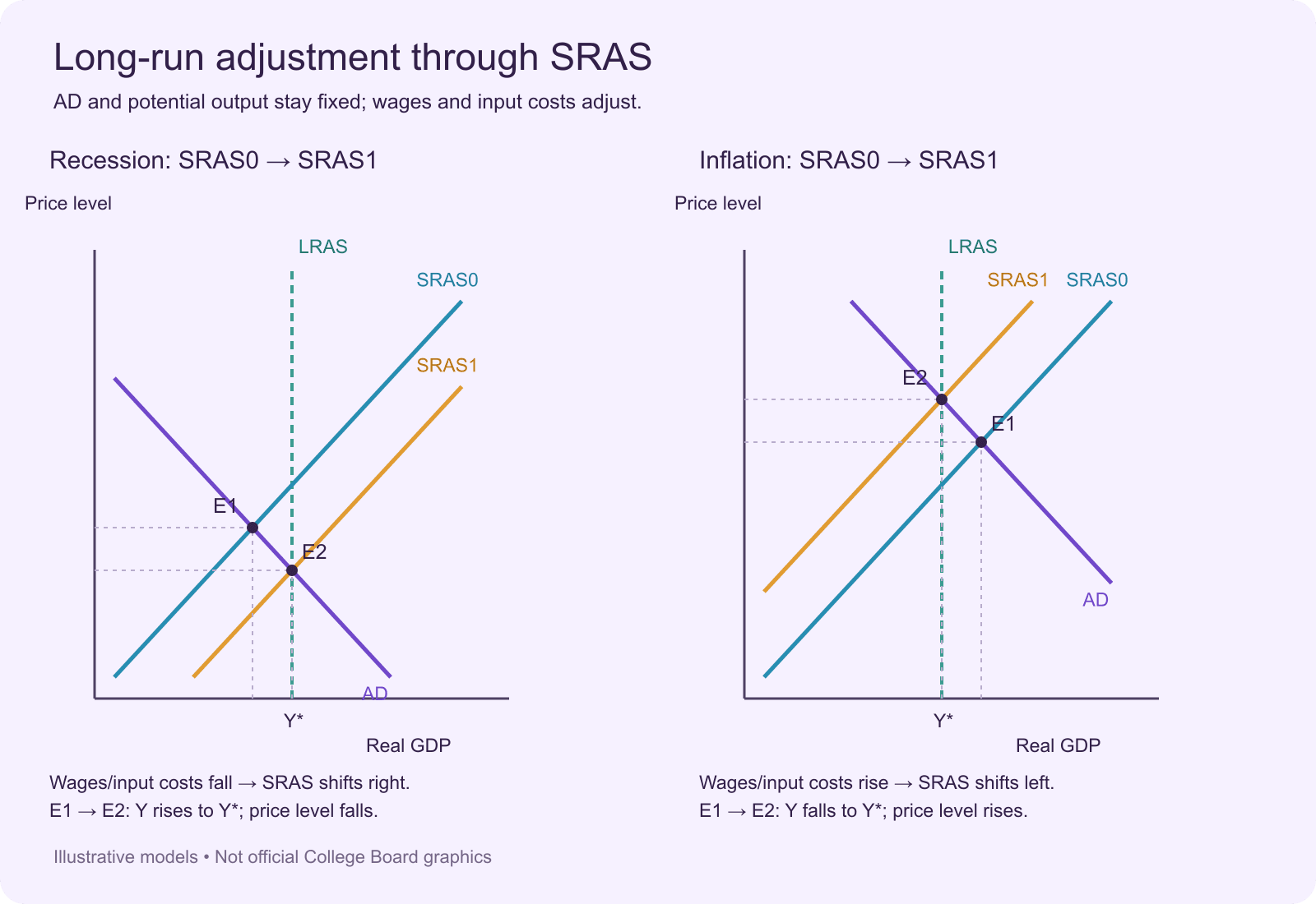
The long-run adjustment process explains how an economy can move back toward potential output after a change in aggregate demand creates an output gap. In the short run, changes in spending or production costs can move real GDP away from its sustainable level.
Over time, wages and other input prices may adjust, shifting SRAS. Understanding this process connects economic fluctuations, price levels, unemployment, and long-run equilibrium.
What Is Long-Run Equilibrium?
Long-run equilibrium occurs when real GDP equals potential output and the economy operates at its natural rate of unemployment. On an AD-AS graph, AD, SRAS, and LRAS intersect at the same equilibrium point.
At this point, the economy has no recessionary or inflationary output gap. Input prices have adjusted to long-run conditions.
Adjustment After a Recessionary Gap
A recessionary gap occurs when short-run equilibrium real GDP is below potential output. Unemployment is above the natural rate because firms produce less than the economy's sustainable capacity.
Over time, weak demand for labor can put downward pressure on nominal wages and other input costs. As production costs decrease, firms may be willing to supply more output at each price level, shifting SRAS to the right.
This adjustment continues until real GDP returns to potential output, assuming no other changes occur. The price level is lower than it would have been without the SRAS adjustment, while long-run output returns to potential.
Adjustment sequence:
- AD shifts left or another shock creates a recessionary gap.
- Real GDP falls below potential output.
- Unemployment rises above the natural rate.
- Wages and input costs gradually face downward pressure.
- SRAS shifts right.
- Real GDP returns to potential output.
Adjustment After an Inflationary Gap
An inflationary gap occurs when short-run equilibrium real GDP exceeds potential output. Firms produce above the economy's sustainable capacity, and unemployment is below the natural rate in the simplified model.
As firms compete for workers and other resources, nominal wages and input costs may increase. Higher production costs reduce the quantity firms are willing to supply at each price level, shifting SRAS to the left.
The adjustment continues until real GDP returns to potential output, assuming no other changes occur. The price level rises as SRAS shifts left.
Adjustment sequence:
- AD shifts right or another shock creates an inflationary gap.
- Real GDP rises above potential output.
- Unemployment falls below the natural rate.
- Wages and input costs gradually face upward pressure.
- SRAS shifts left.
- Real GDP returns to potential output.
Long-Run Self-Adjustment vs. Fiscal Policy
An economy can move toward long-run equilibrium through changes in wages and input costs without new government intervention. This is known as the self-correcting mechanism of the economy.
Fiscal policy offers another approach to addressing output gaps. Expansionary fiscal policy can increase aggregate demand during a recessionary gap, while contractionary fiscal policy can reduce aggregate demand during an inflationary gap.
The mechanisms differ: self-adjustment works through changes in wages and SRAS, while fiscal policy directly affects aggregate demand through government purchases and taxes.
How to Organize AP Macro Unit 3 Notes
A clear note-taking structure helps you connect graphs, formulas, and explanations. Instead of writing every topic as a separate definition, use a consistent format for each concept.
Use a Repeatable Topic Template
For each Unit 3 topic, organize your notes into:
- Definition: Explain the concept in your own words.
- Model: Identify the relevant AD-AS graph or expenditure model.
- Determinants: List the factors that shift the relevant curve.
- Direction: State what happens to real GDP and the price level.
- Example: Add a short economic scenario or calculation.
- Review question: Write a question that requires you to explain or apply the concept.
Keep Graphs and Written Explanations Together
For each AD-AS scenario, include the original graph, the shifted curve, the new equilibrium, and a short explanation. Label the axes, curves, price level, and real GDP clearly.
Do not rely on a graph without explaining the economic event that caused the shift. A short written explanation helps you connect the model to the wording of an exam question.
How to Create AP Macro Unit 3 Notes with Lynote AI Note Taker
AP Macroeconomics students often work with textbook chapters, class slides, recorded lectures, practice explanations, and review handouts. Organizing these materials manually can take time, especially when you need to connect formulas, graph explanations, and economic concepts.
Lynote AI Note Generator helps turn supported learning materials into structured, editable notes. Use it to create an initial study outline, refine important explanations, and prepare materials for review.
Step 1. Upload Your AP Macro Study Materials
Upload supported PDFs, documents, presentations, or recorded lesson files. You can also use supported educational video or webpage links when your material is available online.
For example, upload a Unit 3 lecture about aggregate demand, a PDF explaining the multiplier effect, or your teacher's AD-AS presentation. Use materials you are authorized to process.
Step 2. Generate and Organize Your Notes

Actual Lynote interface; sample content is a generic product demonstration, not an economics lesson. Official source.
Lynote generates structured notes from the supplied materials, helping you group information under headings and key points. Organize the output into sections such as:
- Key Concepts: Aggregate demand, aggregate supply, potential output, and price levels.
- Economic Models: AD-AS relationships and long-run adjustment.
- Important Formulas: Spending multiplier and tax multiplier.
- Graph Explanations: Written explanations of curve shifts and equilibrium changes.
- Unit Summaries: Concise reviews of the concepts covered in your lessons.
Review the generated notes and correct any missing or inaccurate details. Add your own graph annotations, calculations, and worked examples. Lynote organizes the source material; it should not be treated as a dedicated graphing calculator or a substitute for checking economic calculations.
Step 3. Understand Difficult Concepts with AI Chat

Actual Lynote interface; sample content is a generic product demonstration, not an economics lesson. Official source.
Use Lynote AI Chat to ask questions about information contained in your uploaded materials. For example, if your source explains recessionary gaps, you can ask how lower nominal wages may affect short-run aggregate supply.
You can also ask for a comparison of expansionary and contractionary fiscal policy when both are covered in your materials. Check the explanation against your textbook or teacher's notes, especially when a question requires information beyond the uploaded sources.
Step 4. Create Flashcards for AP Macro Review

Actual Lynote interface; sample content is a generic product demonstration, not an economics lesson. Official source.
Turn important definitions, formulas, and economic relationships into question-and-answer flashcards.
Question: What happens to SRAS when nominal wages decrease?
Answer: Lower production costs can increase short-run aggregate supply, shifting the SRAS curve to the right, assuming other factors remain unchanged.
Question: What is a recessionary gap?
Answer: A situation in which short-run equilibrium real GDP is below potential output.
Question: What is the spending multiplier formula in the simple model?
Answer: 1 divided by (1 minus MPC).
Use flashcards to practice recalling concepts, then combine them with graph drawing, calculations, and exam-style questions.
Build a More Organized AP Macro Study Routine
You can use Lynote throughout the course rather than waiting until the final exam review period. Create notes from each assigned reading or lecture, group them by topic, and add your own graph explanations and calculations.
Before an exam, revisit your notes, clarify difficult concepts with AI Chat, and use Flashcards to test your memory. Combine this workflow with official AP resources and practice questions.
Create Your AP Macro Notes with Lynote AI
Common AP Macro Unit 3 Note-Taking Mistakes
Memorizing Curves Without Understanding Shifts
Knowing that AD slopes downward or SRAS slopes upward is not enough. You also need to identify which event shifts a curve and explain the resulting changes in output and the price level.
Better approach: For every shift, write the cause, direction, new equilibrium, and economic explanation.
Confusing a Movement Along a Curve with a Shift
A change in the price level causes movement along an existing AD or SRAS curve. A change in a curve's determinant shifts the entire curve.
Better approach: Identify whether the scenario changes the price level itself or another factor such as consumer confidence, wages, or productivity.
Mixing Up the Multiplier Formulas
The spending multiplier and tax multiplier have different formulas and signs. Using the wrong formula can lead to an incorrect prediction of the change in equilibrium output.
Better approach: Write both formulas on one review card and practice calculations with different MPC values.
Ignoring the Long-Run Adjustment Process
Short-run equilibrium does not always equal potential output. Students should be able to explain how wage and input-price adjustments can shift SRAS over time.
Better approach: Practice the full sequence for both recessionary and inflationary gaps, including the direction of SRAS movement.
Reviewing Definitions Without Practicing Graphs
AP Macro questions often require you to interpret a model and explain a change. Reading definitions alone does not build the skill of drawing and labeling the correct graph.
Better approach: Draw the AD-AS model from memory, label each curve, and explain a new scenario in complete sentences.
Conclusion: Build AP Macro Notes That Connect Every Model
Effective unit 3 ap macro notes connect aggregate demand, aggregate supply, output gaps, multipliers, fiscal policy, and long-run adjustment into one understandable framework. Focus on why curves shift, how equilibrium changes, and what those changes mean for real GDP and the price level.
Organize your class materials, practice graphs and calculations, and review concepts with questions and flashcards. To turn your own lectures, PDFs, and study resources into editable notes, try Lynote AI Note Generator and build a more organized AP Macro study routine.
Frequently Asked Questions About Unit 3 AP Macro Notes
What Is Unit 3 in AP Macroeconomics?
Unit 3 is commonly known as National Income and Price Determination. It covers aggregate demand, aggregate supply, macroeconomic equilibrium, output gaps, the multiplier effect, fiscal policy, and long-run adjustment.
Check the current AP course framework for the exact topic descriptions and exam guidance.
What Should AP Macro Unit 3 Notes Include?
Your notes should explain AD, SRAS, LRAS, short-run and long-run equilibrium, recessionary and inflationary gaps, multiplier formulas, and fiscal policy.
Include labeled graphs, short examples, and review questions that require you to explain how one economic change affects another.
How Do I Make Good Unit 3 AP Macro Notes?
Organize each topic into a definition, model, determinants, direction of change, example, and review question. Keep the graph and written explanation together so you can see how the economic reasoning works.
Review the notes by drawing graphs and explaining scenarios without looking at the answer.
What Is the Difference Between AD and SRAS?
Aggregate demand represents total planned spending on final goods and services at different price levels. Short-run aggregate supply represents the quantity of output firms are willing and able to produce at different price levels when some input prices are sticky.
AD slopes downward in the standard model, while SRAS slopes upward.
What Causes a Recessionary Gap?
A recessionary gap occurs when short-run equilibrium real GDP is below potential output. It can result from a decrease in aggregate demand or another change that reduces short-run output.
In the simplified model, unemployment is above the natural rate.
What Is the Difference Between the Spending Multiplier and Tax Multiplier?
The spending multiplier measures the modeled change in equilibrium output resulting from an initial change in autonomous spending. The tax multiplier measures the modeled effect of a tax change on equilibrium output.
In the simple model, the spending multiplier is 1 divided by (1 minus MPC), while the tax multiplier is negative MPC divided by (1 minus MPC).
How Does Fiscal Policy Affect Aggregate Demand?
Expansionary fiscal policy, such as higher government purchases or lower taxes, can shift AD to the right. Contractionary fiscal policy, such as lower government purchases or higher taxes, can shift AD to the left.
The size of the effect depends on the model assumptions and economic conditions.
What Happens During Long-Run Adjustment After a Recessionary Gap?
When real GDP is below potential output, unemployment is above the natural rate in the simplified model. Over time, downward pressure on wages and input costs can shift SRAS to the right, moving output toward potential GDP.
What Happens During Long-Run Adjustment After an Inflationary Gap?
When real GDP is above potential output, unemployment is below the natural rate in the simplified model. Upward pressure on wages and input costs can shift SRAS to the left, moving output toward potential GDP.
Can Lynote Help Me Create AP Macro Unit 3 Notes?
Yes. Lynote can generate structured notes from supported PDFs, documents, presentations, audio recordings, and videos that you provide.
You can edit the generated notes, ask AI Chat questions based on your uploaded materials, and create Flashcards for review. Check graphs, formulas, and calculations against your original course materials.
Can AI Notes Replace AP Macro Graph Practice?
No. AI-generated notes can help organize explanations and study materials, but students still need to practice drawing, labeling, and interpreting economic graphs independently.
Use your notes as a reference, then practice AD-AS shifts, multiplier calculations, and written explanations.

Written by Hamza Razzaq
Technical Writer
Hamza creates hands-on explainers and technical guides that make AI writing tools easier to understand and use. View all articles →